Foreword
Tying seismic data to well data is an essential step in any QI project. Seismic data are never as good as desired: “zero-phase” and “true amplitude” should never be taken for granted. Although conceptually simple, it relies on many assumptions and is highly susceptible to data quality. This calibration process goes through some form of wavelet estimation. Although there is a wealth of software proposing tools to perform the task, it should never be underestimated both for the time it takes and the difficulty it can represent, all the more that there are several wells covered by the same seismic volume. Sophisticated software and algorithms do not make up for the need to consider the intrinsic complexity of the task.
The point here is not to get into the nuts and bolts of any specific wavelet estimation technique but rather to share a high-level review of its whereabouts and share a few warnings and tips elaborated after a longstanding experience in the subject.
What are we talking about?
I want to consider here the situation where we need to quantitatively assess the transfer function from well derived reflectivities to seismic response; in other words, estimate the wavelet in all of its characteristics.
This is the most elaborated level of seismic-to-well tying as we may consider three progressive levels from the simplest to the more comprehensive and more demanding level:
- Linking well markers / impedance breaks to seismic interpretation,
- Explaining/understanding the shape of the seismic reflectors,
- Explaining/understanding the shape and amplitude of seismic reflectors
Each one of these progressive levels corresponds to different needs and uses of the seismic data:
- Level one is essentially to tie depth to seismic two-way-times (TWT) to build a structural framework allowing the evaluation of bulk rock volumes within structural traps,
- Level two targets finer details od the seismic response as possible clues to understand the sedimentary signature of geological bodies,
- Level three aims at fully comprehend the seismic response usually for quantitative reservoir characterization purposes be it within exploration, appraisal or field description context.
These three levels echo the characterization of the seismic wavelet, the one propagating from surface and through the overburden, having reached the interval of interest and being reflected back to the receiver.
- Level one essentially focuses on the absolute time of the said wavelet whereby it is necessary to evaluate the time delay (or advance) of the seismic energy relative to a time-to-depth relationship provided by borehole geophysics (Vertical seismic profiles or check-shots), At this stage, it is highly desirable to have checked that the data is “zero-phase” (symmetric wavelet, beyond what the seismic processing tells you. This is the key assumption here
- Level two calls for the precise definition of the shape of the wavelet embedded within the data, that is its relative frequency spectrum (both amplitude and phase).
- Level three has the same requirements plus an absolute scaling allowing to generate a synthetic trace that is quantitatively comparable to the actual seismic data it tries to tie with and match. Such a full and calibrated description of the wavelet paves the way to seismic inversion : going the other way around from seismic data as they are to reflectivities and impedances from there on. Mind that it uses is not limited to seismic inversion, it might help directly interpreting amplitudes or relative shape of seismic reflectors, even in a pure exploration context. Seismic inversion is not always the best way to make use of seismic data.
There is a huge body of literature covering algorithms and workflows dedicated to wavelet extraction as depicted in level 3. I shall only refer to Roy E. White, who described a full workflow. In his earlier papers such as “The accuracy of well ties: practical procedures and examples”, [Expanded Abstract, 67th SEG Meeting, Dallas, 1997], Roy E. White advocated that seismic-to-well calibration is a challenging task. As such it requires a careful workflow (data preparation and editing) and dedicated comparison metrics that would turn the well tying exercise from an “art” (eyeball fitting) into a “science”. I fully subscribe to his views related to the need for a detailed workflow with good ness-of-fit metrics.
Typically, the tools used to achieve these seismic-to-well ties are:
- Level1: A synthetic is first generated with a zero-phase wavelet, either parametric such as a Ricker wavelet (a single peak frequency parameter) or an Ormsby wavelet (trapezoidal spectrum defined by four frequencies) or a data derived wavelet such as what is known as a statistical wavelet (derived by a multi-coherency analysis). In most workflows, he key assumption is that the wavelet is zero phase. Most of the time, using a statistical wavelet assumes the subsurface to feature a flat aka white spectrum. Mind the fact that, in case of successive well ties, a prior phase rotation and/or a prior reflectivity color correction can be applied, the validity of which remains to be justified as an assumption. The synthetic trace can be visually scrutinized to identify the desired time shift necessary to match the seismic data. However, this does not yield accurate time shifts and a numerical process such as computing the cross-correlation function between synthetics and seismic traces and identifying the shift delivering the maximum correlation. Mind the fact that such a process can be fairly unprecise, especially when dealing with narrow banded seismic traces and/or prior wavelets for which any unexpected phase rotation in the data is likely to be misinterpreted as a time shift. A tell-tale of a phase error is the lack of symmetry of the cross-correlation function. Displaying this function is an efficient QC of the zero-phase assumption.
- Level2: This level aims at defining the shape of the wavelet. This implies identifying both its amplitude and its phase spectra. In practice, the latter is obtained using the said statistical wavelet while the former is reduced to identifying a constant phase rotation in addition to a time shift -equivalent to a linear phase spectrum whose slope represents the time shift and the intercept the said phase rotation-.Again, the statistical wavelet may or may not take in consideration a possible bias in the well reflectivity spectrum (note that this could be a by-product of a colored inversion workflow). An element of stabilization can be added to this wavelet in way of a spectral smoothing or equivalent to applying a symmetric time function taper (triangular, Hamming, Haning or Papoulis are most commonly used). The phase rotation is usually obtained by scanning a wide range of phase values and identify the phase value, which yields the best goodness-of-fit metrics (usually a correlation coefficient). The natural way to achieve this would be to generate synthetic traces with a range of phase rotation, cross-correlate them with the seismic trace at the well location or in the vicinity of the well bore (hence, also scanning for lateral mis positioning of the wellbore, mis-imaging of the seismic data, fiddling with time-to-depth small variations or finding better conditions for the tie) and pick the one combination that maximizes the fit. A very efficient way to do this is to compute the envelope of the cross-correlation, find the time of its maximum for the time shift and derive the instantaneous phase at this precise time, from which the optimal phase rotation is obtained. A not-so-small detail flows from the way the cross-correlation function is centered. Some software centers it (equivalently defines time zero of the wavelet) at the positive peak whereas others center it at the maximum of its envelope. This practical detail is not so innocuous when applying a taper function symmetric relative to the time origin since it would distort the relative shape of the cross-correlation side lobes and bias the resulting phase. Mind the fact that the former choice shall produce a residual linear trend in the phase spectrum, which may lead to misinterpreting it: the constant phase rotation needs to be read at the intercept of the linear trend and not at the peak frequency of the amplitude spectrum. It is also worth oversampling the cross-correlation function to get better precision (considering that the time series fully rotates its instantaneous phase within a time period-360 degrees within a 1/dominant freq time span, defining the maximum of a 30 Hz dominated time series at a 4ms sampling rate would lead to a +/- 20 deg uncertainty: useless to qualify a phase value with decimal places).
- Level3: Here, the objective is to get rid of all the aforementioned explicit assumptions used at the previous levels (linear phase, color of the subsurface reflectivity and directly estimate the wavelet using a numerical inversion scheme. Such schemes compute the wavelet (aka filter) that relates the output (seismic trace) to the input (well derived reflectivities) minimizing a cost function essentially consisting of the residual energy (Least squares case). Consequently, the output wavelet is also calibrated in amplitude (aka gain). There are many such algorithms which work either in the time or in the frequency domain. Like any numerical inversion scheme, additional constraints are usually added to get a stable solution (the wavelet), which one should consider as implicit assumptions. In addition, one should keep in mind the basic but essential assumption that the convolutional model applies. This assumption fails when the seismic data still contains multiples or reflectivities in strongly heterogeneous media at large incidence angles are considered: what some algorithm would consider as plain data errors could very well represent our inability to correctly represent the full complexity of the seismic wave propagation.
Apologizing in advance to the most experienced geoscientists, let me insist here on a few tips, which might be found obvious.
Ahead of the well-tie. Data preparation
The mere fact of considering reflectivities to compute a synthetic trace from well data implicitly assumes that the convolutional model applies. As such, because of linearity, all sampling rates should yield consistent synthetics: for example, decimating (1 in 10) a synthetic trace computed at a 0.1 ms sampling rate should give amplitude samples identical (within numerical accuracy) to those directly computed with reflectivities computed at a 1ms sampling rate provided the wavelet’s frequency spectrum does not contain energy above 500Hz in theory (sampling theorem – Shannon) or 250 Hz in practice. Such a property guarantees that the process of reflectivity computation is flawless and is consistent with the generally accepted convolutional model. Such a behavior requires applying an anti-alias filter to well based impedance data naturally sampled in depth at a very fine sampling rate before computing reflectivity at a much coarser sampling close to the seismic sampling rate. Should the computation be performed first at a very fine sampling rate, the final decimation step should involve a scaling of reflectivities (factor of ten in the case of a 1 to 10 decimation) to get consistent amplitudes. Indeed, missing such a scaling can easily be compensated by a stronger wavelet. However, this becomes important when quantitatively comparing different software and workflows.
In addition to the necessary sonic and density well logs, you might want to consider any additional log informing you of the quality of the wellbore such as the caliper log. Caliper (and resistivity logs) should also point out reservoirs potentially invaded by the mud fluid: oil-based muds can invade permeable aquifer as much as water-based mud can invade hydrocarbon bearing reservoirs. Because of density and compressibility differences between formation and mud fluids, density and sonic logs might record different properties in the immediate vicinity of the well bore. Such modified properties will be “unseen” by seismic data. In those cases, entering the world of fluid substitution, shear wave sonic and AVO (Amplitude Variation with Offset) might become necessary. In the case of producing field, you might experience the impact of production (pressure and fluid substitution) on those elastic parameters. Keeping track of the calendar of operations (seismic acquisition vs. production) could prove useful.
Talking about Shear wave logs, it is good practice to display Poisson’s ratio (PR) or Vp/Vs ratios next to P-wave sonic and density rather than S-sonic. As a matter of fact, this is a pragmatic way to track errors in either P- or S- log data. Those would show as extreme PR or Vp/VS values (negative or too high for the range of burial). In addition, large contrasts in those should point out places where strong AVO could occur and acquisition undershoot becomes an issue.
Mentioning elastic log display (rho, P- and S-velocities), it is also an even better practice to represent densities, P-sonic and Vp/Vs on logarithmic scales or their logarithm transforms on linear scale. The rationale for this is straightforward since reflectivities are the relative changes in impedance. Relative changes are robustly approximated (Delta(Z)/2Z ~1/2 Delta(Log(Z))) and therefore be visually assessed by the absolute differences of the log values. That is to say that the deflection of the logarithmic values between two lithologies is approximatively proportional to the reflectivity between them. This approximation is very robust. This is all the more relevant that Log(Impedance) =Log(density)+Log(velocity): the contribution of density relative to that of the velocity should stand out if the linear scales used to display those logarithmic transformed data span intervals of the same length (Same Vmax-Vmin). In addition, Log(Vp/Vs) appears in proxies to reflectivities at non normal incidence. Such a method of display is certainly unfamiliar to the petrophysicists. However, this is one that is the most appropriate to the ones concerned with understanding what the seismic response is made of.
Tying angle/offset substacks (as used in AVA/AVO studies (Amplitude versus Angle/Offset) to well data opens up a whole range of specific difficulties, well beyond shear wave reliability or even availability. The first thing is to make sure the “pre-stack” seismic data (aka seismic gathers) is processed in a way that delivers more or less correct angles, which can be challenging when VTI (Vertical Transverse Anisotropy) is present in the overburden. The second thing is that the use of reflectivities assumes a linear or convolutional model. Whereas the amount of reflectivity of a single interface between two semi-infinite homogeneous media is well known. It was theorized by Karl Zoeppritz in “On reflection and transmission of seismic waves by surfaces of discontinuity”[News from the Royal Society of Sciences at Göttingen, Mathematical-Physical Class, 1919]. It must be considered as a high frequency approximation. When applied at practical seismic bandwidth, the media on either side of any contrast is highly unlikely to be homogeneous. In other words, applying Zoeppritz’ equations between any time sampled rock properties violates the basic hypothesis underpinning these equations. Mischaracterization of the reflected amplitude shall be more pronounced at larger angles and for stronger contrasts. A proxy to these equations has been proposed by Keiti Aki and Paul G.Richards [Quantitative seismology: Theory and methods, vol 1, p 153, 1980], leading to the concept of elastic impedance, which reduces some of the artifacts but remain an approximation.
In some situations, tying a “full stack” as an acoustic-only response (i.e. using P-wave velocities and density) might reveal tricky since the inclusion of larger offsets in the stack of amplitude might be sensitive to AVO anomalies (commonly expected at hydrocarbon reservoir boundaries). In absence of shear wave data, it might be advisable to tie an AVO intercept (in theory) or a near angle/offset substack to estimate wavelets notwithstanding its greater susceptibility to internal multiple residuals
Similarly, you want to consider seismic acquisition conditions. Surface obstructions (typically a rig present while shooting seismic data) usually lead to undershots. Larger offsets are then used to fill-in the gaps. Because of the way onshore data are shot, there are huge variations in fold and offset coverage that modifies signal-to-noise (S/N). This is where scanning laterally to the well head becomes necessary. Besides fiddling with uncertainties, the point is to locate places with the best conditions for wavelet extraction. To help understanding goodness-of-fit maps, it is good practice to keep an eye on a satellite image when onshore and a shallow time slice. Onshore or transition zone are the most prone to weird looking wavelets.
You might want to check well locations in your database. Hopefully in rare occasions, long standing projects might have endured geodetic reference changes leading to large projected horizontal displacements. Well trajectory measurements have undergone major improvements through time. Older wells might have quite uncertain trajectory especially in areas closer to the poles.
In the case of missing density. Information, it is customary to fit an exponential law relating density to sonic, the so called “Gardner’s law”. Most of the time, people would fit at log scale. In the general case, there is no reason why the same relationship would hold at all scales (self-similar aka-fractal behavior) across geological periods with highly variable depositional context. It might be more relevant to perform the fit at scales relevant to the seismic scale. In the special situation where density is missing across the whole sonic interval. Mind the fact, that using the same Gardner’s parameters across the entire range only impacts reflectivity by a scalar (1+ Gardner’s exponent) (check it via the logarithmic proxy to reflectivity). This has only relevance when amplitude match is sought for (level 3). It would not change results at level two.
Additional data
Even though borehole geophysics became less fashionable with time for economic reasons (The cost of Vertical Seismic Profiles aka VSP’s tend to be saved in well data acquisition programs), one should not forget about such data when available (especially earlier exploration wells). Bear in mind that this is the only experiment performed at seismic scale, which is both in depth and in time. Through processing, the “Corridor stack” is, in theory, an ideal experimental version of the band limited reflectivities. As such, it is good practice to compare corridor stacks to well synthetics for QCs. Significant differences should prompt for a second look at well log data and/or VSP data (from which the time-to depth is extracted).
Using corridor stacks usually provides TWT intervals much larger than well logged intervals. Large intervals should help stabilizing wavelet extraction algorithms (more redundancy). They should also allow for the lower frequencies missing from shorter log intervals.
In specific situations where the borehole terminates at geological breaks with strong impedance break (e.g. top basement, top carbonates) the ability of the VSP to record band limited reflectivities below the well TD (Terminal Depth) (so called vision “ahead of the bit”) can be a definite advantage, all the more that seismic data feature very strong amplitudes, hence a very good Signal-to-noise ratio (SNR).
Some consequences of numerical processes
More than often, the numerical processes described above involve some cosmetics to deliver stable parameters (levels 1 and 2) or a stable (aka nice-looking) wavelet (level 3). Indeed, some form of spectral smoothing or time function windowing/tapering shall help delivering stable wavelets. It must then be born in mind that such processes favor zero-phase appearance and the onset of a non-realistic DC component (non-zero average amplitude or energy at zero frequency).
Too much cosmetics as evidenced by a strong DC component of the wavelet deprives oneself of the ability to evaluate the quality of the data (either seismic and/or well data) not highlighting inconsistencies between the two sources of data, which would yield unstable (poor-looking) wavelets otherwise. Many commercial software has default options whose objective is to yield a stable wavelet blurring the perception of data quality to the interpreter’s view.
On a different standpoint, least squares approaches tend to deliver weaker wavelets when the quantitative tie with seismic data is poor. This is perfectly understandable since the gain to be applied to any given wavelet (or to the resulting synthetics) can be easily solved by minimizing the residual calibration energy, which is a quadratic function of the gain. The optimal scalar to be applied to the given wavelet shape is simply the ratio of seismic RMS to synthetic MS weighted by the correlation coefficient It is easily obtained by linearly regressing the series of seismic samples as a function of those from the synthetic trace provided a time match has been made with a satisfactory waveshape (i.e. amplitude calibration -level3- depends on the time -level 1- and the phase -level 2- matches).
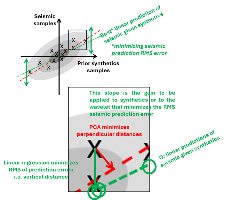
Poor ties shall have a low correlation, hence a low gain. Balancing synthetics RMS to that of the seismic data either by display or by artificially boosting the amplitude of the wavelet tends to hide the fact that the tie is poor.
At this point, we understand that the task of quantitatively estimating a wavelet from seismic data (level 3) can be very challenging. In addition to many of the pitfalls, some of which have been described above, any algorithm shall deliver a numerical solution, sensitive to its internal parameter such as wavelet time length, amount of frequency smoothing, type of time tapering, length of the data (to provide redundancy), presence of seismic or geological frequency notches, to only name the most common ones. When too unstable, it is better to reduce the ambition of the task (level 3 to level2 for instance) which amounts to make more hypotheses and reduce the number of parameters to be estimated (from wavelet’s amplitude samples to a single phase rotation applied to a predefined statistical shape)
Even though the use of goodness metrics (correlation, RMSE, ….) might make the process appear as a “science”, it must be acknowledged that it remains an “art” where common sense and experience are more important than the piece of software used.
Multi-well issues
This aspect becomes even more important when several wells are available. In such situations, it is not uncommon that wavelets, although carefully crafted/estimated at each individual well, are significantly different. The problem becomes which wavelet to choose (in seismic inversion projects or to present all synthetics with a wavelet comparable for say) or how do I come up with a single wavelet?
Practitioners use a variety of different strategies. The most common one consists in averaging individual wavelets. This is no trivial matter.
Firstly, there arises the issue of taking into account the zero-time (aka convolution origin) of each individual wavelet. In other words: how should each one of the wavelets be synchronized? This question flows from the fact that time references are relative to the seismic data time origin (and Check-shot time origin. The latter is usually assumed stable, at least with marine data, less so with onshore data (near surface statics). The former can be a bit floating since this is the result of compound corrections (rig elevation relative to some reference, measurement delays), VSP processing, first arrival definition (picking maximum energy, or impetus, before or after deconvolution… all very much dependent on the contractor who recorded and processed the borehole seismic. Wells are most likely of different years and therefore different contractors, implying that there is no absolute time reference to cling to. Keeping in mind that the objective is to come up with a single wavelet, only relative differences are to be resolved. Should all the wavelets have the same shape, this would be easy. However, when wavelets have different shapes, should the relative delays be deduced from the onset of the maximum amplitude of from the maximum energy or envelop? I am not aware of any theoretical answer to this issue and this is down to individual’s preference. This issue relates to the depth corrections applied when mapping time structures. When examining QI contractor wavelet displays, pay attention to where time zero of each individual wavelet display falls relative to the wavelet characteristic shape. This would be representative of some strategic choice made by the contractor “behind the scene”.
Secondly, how should amplitudes be handled through the averaging process? Should wavelets be normalized before averaging or should they be weighted according to some factor such as their energy, a seismic data RMS measurement, or their goodness of fit? Considering the last option, should an excellent tie (world class correlation coefficient) be given the same weight than a mediocre one, irrespective of the underlying seismic energy at their respective well location. In case of a seismic inversion project, such a strategy would not deliver an averaged wavelet that minimizes residuals globally (across all the wells). When examining QI contractor wavelet displays, pay attention to the amplitude scales, was there some normalization applied? Only for the display or to the internal numerical entity? This could be representative of some strategic choice made by the contractor “behind the scene”.
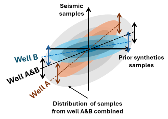
The figure above illustrates the difficulty or dilemma when trying to define a single amplitude (or wavelet gain) from two wells whose best amplitude match is very different from the individual ones, assuming the two synthetic traces are using the same wavelet. Interestingly enough it shows that even if those two wells yield synthetics that correlates very well with their local seismic data, the bundling of the two wells in a single least squares (LS) amplitude estimation process might deliver a much poorer overall calibration/correlation. In this sketchy example, one can understand that keeping as good a correlation as the individual ones requires locally correcting seismic amplitudes beforehand. This simple example also illustrates that the optimal LS gain would correspond to taking the average of the two wavelets when the RMSes and correlation of the two synthetics are comparable. Other situations are no trivial matters and would most likely lead to optimal solutions than simply taking the average. Normalizing the wavelets before could be one strategy whereas taking the individual seismic and synthetics amplitude distribution would be another one.
Stable or not stable wavelet ? : that is the question
In reality the key issue when facing different wavelets at different locations is to decide whether the seismic data can be efficiently and correctly characterized by a single wavelet (differences are only apparent ones and are due to the intrinsic instability of the wavelet estimation) or if seismic processing was not able to process the data in a way that correct for genuine lateral variations thereof. There could be many reasons causing such variations impacting the frequency content, phase spectrum or amplitude of the wavelet. Onshore data may feature lateral variations, which modify the way the physical source (explosives or vibrator) interact with the near surface: hard-compacted-rocky/soft- loose sediments ductile/brittle soil (e.g. salt, sand dunes), nature/thickness of the weathered zone, depth of the water table, … Marine data should not exhibit such issues. Transition zones are likely to be impacted by bathymetry. In addition, the complexity/heterogeneity of the overburden might transmit the seismic energy differently.
Deciding whether the data can be characterized by a single wavelet is often an act of faith and truly more an “art” than a “science”. As a matter of fact, it is much more comfortable to believe and consider that there are no lateral variations, which generally is a key hypothesis for many QI workflows and software applications. However, it should be reminded that absence of evidence is not evidence of absence.
QQC maps as an aid to seismic wavelet estimation
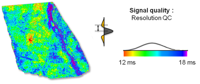
This where Quantitative QCs (aka QQCs) should come in and provide hints if not clues to the existence of lateral variations. QQCs means the mapping of seismic attributes derived from thick intervals for which geological properties are expected to be stationary either deterministically of statistically. Attributes should strive to characterize frequency content (e.g. thickness of the central peak of the auto-correlation function), energy (e.g. RMS of amplitude samples). Whenever available, cross-correlating angle stacks can provide additional attributes such as correlation coefficient, relative phase differences between angle stacks. The mapping of these attributes is a very powerful tool to help decide if variations are randomly distributed or aerally organized.
The next figure adapted from Alexandre ARAMAN and Benoit PATERNOSTER in “Seismic quality monitoring during processing” [First Break volume32, 2014] is an example of such a map. In particular, this seismic time resolution map highlights areas with a much higher frequency content than surrounding areas. Assuming geology is stationary across the QC interval that was used, a well located within a hot color area is more likely to deliver a higher frequency content than elsewhere, also potentially noisier (to be checked with other maps).
It is much more efficient than checking a bunch of test lines. In effect, those maps can help selecting test lines for processing tests based on their representativity of the observed variations. Interpreting those maps can be tedious and complex as attributes are different symptoms of the same propagation complexity. They tend to be linked one with another (e.g. amplitude variations can be the consequence of variations of the frequency content or not).
In addition, one should not forget about taking advantage of peculiar geological interfaces or layers. The simplest of all is the sea bottom interface in deep offshore data. It is generally a strong impedance positive contrast, sometimes sufficiently isolated from nearby reflectors to allow the characterization of the wavelet shape (or phase), at least at the top of the sedimentary pile. Deeper volcanic intrusions can take the form of thin (relative to the seismic wavelength) and very hard layers. Maximum flooding surfaces, a top carbonate, thin shallow gas accumulations, top or base salt, anhydrite layers linked to thick evaporite deposits are examples of geological situations that can provide reference reflectors of constant amplitude and/or shape. Regional geological knowledge should be taken in consideration.
The use of specific geological situations to be used as seismic reference or yard sticks for wavelet characterization echoes the message delivered by Alistair Brown in “Phase and Polarity Issues in Modern Seismic Interpretation” [Search and Discovery Article #40397 (2009)].
The limited sampling of the well data delivering deterministic wavelets should be completed by the comprehensive mapping of QQC attributes whose relevance is more statistical than deterministic. Posting characteristic features of wavelets obtained at well locations onto such attribute maps can help understanding lateral variations and deciding if individual wavelets can be blended into a single one.
Scrutinizing such QQC maps prior to the exercise of seismic-to-well tying help anticipate difficulties and prioritize the work. For instance, a map representing the seismic bandwidth should tell which well has the best potential for determining the seismic phase or a map representing the correlation between angle stacks should tell you which area has a better SNR, favorable to a robust wavelet estimation.
Lastly
Ultimately, reliable seismic calibration requires blending multiple data sources with a dual approach. Managing these complex workflows is not just a matter of following a technical recipe, but rather an ongoing balance between scientific rigor “science” and the intuitive judgment gained through experience “art”.