Foreword
Offset-to-angle mapping is one of these processing steps, which appears trivial and and taken for granted. However, it is very often overlooked and can be the source of pitfalls. When its whereabouts are correctly understood, range it is fairly easy to perform in most situations. This processing step is one of the final processing steps before the processing tean delivers the data to its client/interpreter. This is a unique opportunity for a final dialogue between the two parties: How did the data quality came out from processing ? What is the useful offset range that is safe to use for QI ? How shall the output data be used (attribute extraction, seismic inversion) ? which is the interval and area of interest for which the angles should be careful designed ?
It turns out that many projects are running out of time: Processing lags behind schedule or is very close to its deadline, interpreters have their own short deadlines to meet (delivering an interpretation, a prospect evaluation, a well target, etc.). Consequently, there is too often very little time to discuss alternatives, methods, parameters, etc. despite the fact that these choices (likewise any processing parameter) shall impact month-long projects if not years.
It is therefore important to know and understand the whereabouts of this process to be able to timely raise the correct question to the processing Team /supervisor.
The length of this article and the details it contains might surprise even seasoned QI practitioners. Most of them are often overlooked as this process is usually taken for granted and left to the processing team’s judgement. Nonetheless, experience taught me how important they can be.
What are we talking about ?
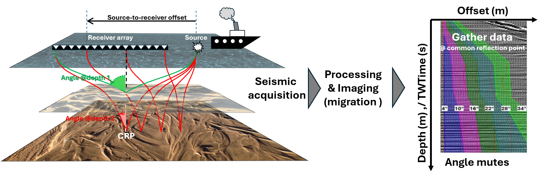
Seismic acquisition and most processing steps are performed in the offset domain whereas, propagation and reflectivities involve incidence angles. When it comes to quantitative interpretation, it is important to know at which incidence angle corresponds any given time/depth and offset pair. Furthermore, when QI deals with so called pre-stack data, be it AVO intercept and gradient or angle stacks (stack of amplitudes recorded within a given incidence angle (specified by two angle mutes), calibration, interpretation, inversion are much dependent on the angle definition.
In principle, this is not a difficult matter as long as subsurface velocities are known, which is always the case at this late processing stage via stacking velocities when dealing with legacy time processing or via migration or even full waveform inversion velocities when dealing with modern depth imaging. In practice, there are a few subtilities in the choice of seismic velocities, their nature and quality, in the selection of the computation method and its angle definition.
Angle mutes should be defined such that the offset geometry fully covers its range within the interval and area of interest (AOI). Caution should be exercised with legacy angle stacks, whose definition was (hopefully) appropriate for the target they were supposed to cover when they were first generated. Such a definition might not be adapted for different targets (e.g. deeper or different prospect). Further, legacy (and fairly old) data might have been computed using simplified methods.
This is important, since nowadays seismic projects tend to cover very large areas so that many seismic datasets are assembled from the merging of existing substack datasets whose angle definitions possibly differ one from another. Should such project undertake the merging from raw data for the sake of The lengthharmonization and benefit of modern processing / imaging tools, different geometries are likely to co-exist (streamer length, source-to-streamer distance i.e. maximum and minimum offsets). Those should be accounted for when designing angle stacks.
What are the most common techniques ?
Early substacking techniques involved splicing the gather in offset ranges, leading to angle variations from top to bottom. Improvement came with the splicing of the gather acording to the processing mutes (inner and outer), which supposedly isolated the better part of the data.
Then the use of techniques aimed at actually defining angle ranges using a velocity model. With a perfect and fully described velocity model, ray-tracing would be the logical choice. There are many ways to ray-trace through a subsurface model depending on how it is numerically represented. Subsurface can be modeled as a 3D grid of velocity values, a succession of layers of constant velocity bounded by dipping interfaces or a mix of these sometimes with dips being defined from the seismic data themselves. However, it must be considered that ray theory is a high frequency approximation. In order to reduce the sensitivity of ray-pathes to inputs, smoothing is necessary. To my knowledge, the amount of smoothing is arbitrary and based on educated judgement.
In his 1991 paper « Making AVO more robust », Walden proposed what I consider to be a smart formula to derive incidence angles. Assuming an isotropic layer cake subsurface and moderate angles, the formula can be easily demonstrated.: As long as the two-term normal move out (NMO) equation holds (roughly 30 degrees), it represents the wavefront curvature at the surface as it varies along the receiver array (i.e. as a function of offset). This equation is only driven by two parameters: To (TWT at zero offset) and a stacking velocity Vstack at To. The equation can be differentiated relative to the offset variable to get the apparent velocity of reflector at To when it hits the receiver array at any given offset. The apparent velocity at the near surface is a simple function of the emergence angle and velocity of the first layer. The flat layer assumption allows using Snell-Descartes’ law to backpropagate the emerging angle at the surface all the way down to the reflector at time To and relate it to the incidence angle at depth using the local interval velocity Vint. Once the algebra is carried out, the final formula looks as if the reflector’s overburden is a homogeneous medium of velocity Vstack , through which a straight ray approximation delivers a crude incidence angle via geometric considerations. Considering the velocity right below the interface to be Vint, Walden’s result would correspond to the angle right below the reflector. This simplistic interpretation of Walden’s formula does not honor its physical meaning and probably contributed to a perceived over-simplistic equation grossly inferior to a ray-tracing solution.
The smartness of the formula resides in the fact that you don’t need to apply reccursive formulae through a fully described model; All is needed are Vstack and Vint profiles as a function of TWT. Once defined, it is easy to go from offset to angle and vice versa.
Under the layer cake assumption, Vstack is equivalent to Vrms. Vint (TWT) can be computed from Dix’s formula.
Walden’s formula is well adapted for compaction driven velocities (e.g. deep offshore basins) whereas significant lithology variations (e.g. carbonates/salt) and marked structural regimes might require ray-tracing techniques.
Once incidence angles are computed for any depth or TWT and any offset, amplitudes from gathers can be used to derive AVO intercept and gradient or to define isoangle lines through the gather to derive substacking mutes
When comparing seismic datasets in angle, make sure you know its design : inner/outer mutes, parameters, velocity input, computation method are comparable at the risk of comparing apple with oranges. Always refer to the processing report
Walden’s formula in practice
Although the hypotheses underpinning the derivation of the formula are clear, this equation is fairly robust when applied to simple structural situations and geological environments whose velocity profiles are compaction driven.
It is true that at large offsets leading to large incidence angles, the formula tends to overestimate angles relative to ray-tracing by only a few degrees (even in the 40-50 degrees range). However the direct mesurements of incidence angles using walk-away acquisitions (polarization analysis of direct arrivals at downhole three-component geophones) is well accounted for by the formula except in anisotropic situations. Differences between measurements and their numerical predictions are comparable to the measurement variabilities.
Because it is based on the actual kinematics of seismic waves, it is more likely to reproduce incidence angles applicable to the seismic bandwidth whereas applying ray theory (a high frequzncy proxy) to a subsurface model whose despription is based on high frequency details (interfaces, reflectors) is more susceptible to generate irrelevant results. As a matter of fact, in compaction driven basins, isovelocity surfaces derived from kinematics tend to mimic seabed even if seismic reflectors, sensing the higher frequency content of the subsurface properties, often show structural features not comformable to the seabed. In other words, the gradient vector of velocity spatial variations varies with frequency, hence, ray-tracing through a subsurface model based on reflectors is likely not to apply to the kinematic behavior of the seismic waves, sensitive to the lower end of the seismic spectrum.
Time processing and imaging workflows generate velocities of the same nature as stacking velocities. Thus deriving interval velocities using Dix’s formula is required. Unfortunately, this process is very sensitive to errors in the input velocities. Vertically and horizontally smoothing stacking velocities is not the most efficient way to produce stable interval velocities required by the formula. It is therefore preferrable to directly smooth interval velocities, from which RMS
A word on VTI anisotropy
Tips for QCing offset-to-angle transform / parameters to watch for
In Walden’s formula, the Vint/Vrms ratio would be the source of instabilities: Vrms is usually very smooth and laterally stable while Vint is very susceptible to small errors. In order to QC velocity fields to be used for an offset-to-angle transformation, images of this ratio can prove useful to identify angle mute spurious swinging in the offset domain. Mapping this ratio at target level to point out areas of suspicious variability could be an efficient QC prior to any AVO analysis.
When scrutinizing an isolated reflector from an offset gather with posted angle mutes or from different angle stacks. The reflector is stretched in time at larger offset/angle. The amount of stretching increases with offset/angle. As a matter of fact, the amount of absolute stretch is a function of structural dip and angle of incidence. The relative stretch between near offset traces and far offset traces is solely driven by the incidence angle. It varies as 1/cosine(angle). This implies that, for say, at 60 degree of incidence, the reflector should nominally be twice as thick as it is at near offset/angle : 60 dg => 200%, 45 deg => 140%, 30 deg => 115%.
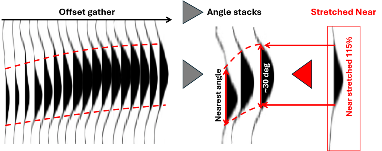
When applied to a single gather display as in the above illustration, this is only an approximate control of consistency. The same idea can apply to time resolution maps computed from existing angle stacks (from Quantitative QC’s aka QQC -see Araman & Paternoster in TLE). Time resolution ratios maps should statistically match the theoretical relationship, unless some post-processing had been applied.
Incidentally, the Vint/Vrms ratio can be considered as a correction applied to a straight ray incidence proxy to get a curved ray incidence angle. Namely, this ratio is applied to sin²(incidence_straight-ray). Because Vrms varies smoothly with depth/time, back and forth swinging of mutes are indicative of velocity variations. Moving backward (forward) – toward smaller offsets as depth/time increases indicates an increase of velocity (respectiveliy decrease). When controlling mutes from sampled gathers, it is good practice to check the offset’s lows and highs with major geological formations.
In previous sections, the importance of interval velocity smoothing was highlighted. In the case of high velocity formations( e.g. carbonate, salt) the high velocities shall be smeared and bias the lower velocities of the over- under-burden. Should the target be close to these formation boundaries, amplitude attributes might be biased too as it gets closer to the boundary (e.g. dipping reservoir below base of salt), potentially messing an updip/downdip comparison when analyzing DHIs.
Such situations also produce large variations in fold. In order to prevent this, some software implements a so-called « protection » preventing offset values along a given angle mute (sharply reducing the fold) from decreasing as depth/time increases (« outer mute protection » aka « salt protection »). querying if this option has been activated or not is good practice.
Furthermore, for those analysing AVO using the intercept and gradient attributes extracted from gathers, it is worth noting that their Least squares estimates (aka linear regression of amplitudes as a function of sin²(incidence angle)) are nothing but a weighted sum of the gather amplitudes within the selected angular aperture. These weights are function of the sin²(incidence) of each individual amplitude. As result, the AVO gradient can easily be modified from a straight ray proxy to any curved ray computation honoring the same Vrms by a simple (Vint/Vrms)² factor.
Mind the fact that such a factor is unlikely to justify the factor sometimes applied to gradient to « scale » a real data Gradient/Intercept crossplot slope to that of a modeling.
Vertical sampling of the velocity data
Modern software nowadays accomodates finely sampled velocity fields. There remains the necessity to watch for too coarsly sampled velocity fields (from legacy data for instance). Time processing /imaging workflows consider velocities of the same nature as stacking velocities. Those velocities are analogous to RMS velocities. As such, their vertical variations are smooth and they do not need to be finely sampled. However, turning them into interval velocities is analogous to taking a vertical derivative. , thus generating much more rapid variations. Those rapid variations require a finer sampling to be correctly characterized. Hence, the vertical sampling of a time migration or stacking velocity field should be finer than what appears necessary to ensure a correct sampling of interval velocities.
Using too coarse a velocity sampling shall generate a significant leap backward to any angle mute right at each velocity sample. Such a sharp change in the muting is likely to produce odd (breaks in waveform) results on any amplitude based attribute extraction.
Tapering below mutes
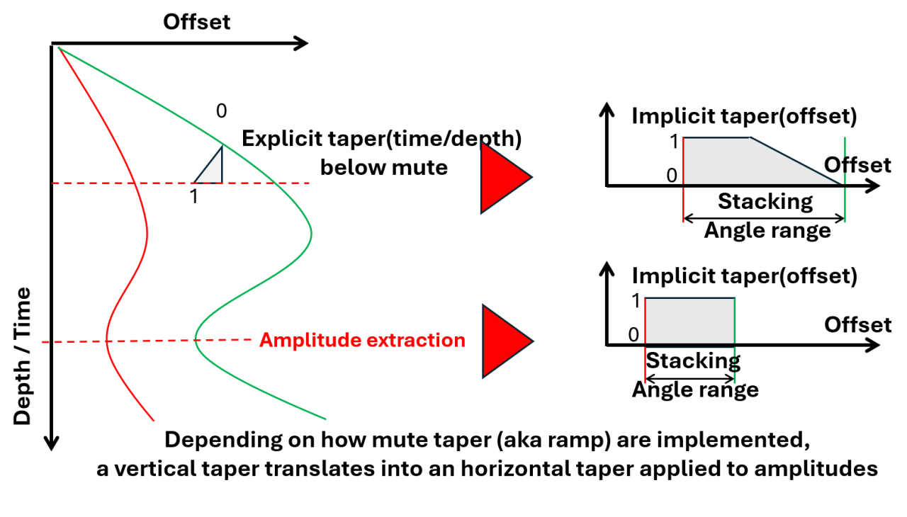
It is common practice to apply an amplitude taper attached to mutes. It is preferrable to use minimal tapering since any taper shall damp amplitudes within the range of offset/angle to be stacked. A long taper would bias the amplitude output towards the smaller offsets and lower angles of the range. Furthermore, if there are significant velocity variations, the mute shall swing back and forth. The varying slope of the mute shall induce a variable angle bias in the output.
How to select inner and outer angle mutes?
Now that we know how angle mutes are computed and what are parameters to watch for, it is time to discuss the choice of incidence angles that shall drive an inner and an outer mute between which prestack amplitude attributes shall be exptracted for AVO or inversion studies: AVO intercept/gradient or angle substacks.
Because minimum and maximum offsets have values constrained by acquisition parameters, not all incidence angles are recorded at all depths: the deeper your target is, the more limited the maximum angle shall be; the shallower you go, the more restricted the minimum angle shall be.
Prestack analysis is very sensitive to noise. AVO intercept/gradient are most sensitive to the angular aperture (both sides); Near and Far angle stack comparisons are sensitive to incidence variations. Irrespective of the desired analysis technique to follow processing output, it is essential for the robustness of any prestack analysis that angular apertures remain consistentthroughout the area and depth of interest in order to ensure that observed relative variations are comparable from one area to another (updip vs. downdip / one sand fairway to another).
The top of the interval of interest shall drive the selection of the inner mute or minimum angle while its bottom, the outer mute or maximum angle. Because subsurface usually feature lateral velocity variations and targets cover different structural positions (from structural Apex, potentially hydrocarbon (HC) filled, down to spill point, potentially transitioning from HC to brine), the mapping of the minimum and maximum angles are highly recommanded to decide for these cut-offs. Namely, selecting the largest value reached by the map of the minimum angle and the smallest value of the maximum angle throughout the AOI would ensure the available offset range allow the amplitude extraction across this selected range of inner and outer mutes. In this way, angular apertures shall be consistent through the AOI .
Such a selection might reveal quite restrictive when applied to a large exploration area. Thus taking an accurate account of actual targets and interpretation whereabouts might be necessary to keep a sufficient incidence aperture. Mapping faiways and potential traps onto these angle maps is a good practice.
This workflow greatly benefits from the simplicity and directness of Walden’s formula. The formula can be applied directly using map extractions of interval and RMS velocities, once time grids of the top and bottom of the target interval and maximum offset are available.
This is precisely when and where interaction between the seismic processing team and the final client / interpreter should occur: minimum/maximum offset should be understood as minimum/maximum « usable » offsets from the gather (rejecting internal residuals multiples / possible « garbage » at larger offsets); only the clientknows the interpretation stakes precisemy enough to accurateley define the AOI.
There is no one-parameter-set fits all angle design
This also stresses that there is no one-parameter-set-fits-all angle design. Parmeters should be carefully designed according to the objective and the data themselves. Using legacy datasets (AVO intercept/gradient pair or Near/Far) without knowing why and how they were designed paves to way to misinterpretation. Access to a detailed processing report is a must when dealing with legacy data. Be particularly suspicious when angle stacks are a « standard » 0-15/15-30/30-45 degrees
Which angle to assign to an angle range?
When stacking seismic amplitudes between inner and outer mutes (aka setting minimum and maximum angle cut-offs to generate so called « angle substacks »), it is convenient to assign a single incidence angle value to the generated piece of data. It is common practice to assign the average of the two angles.
However, especially if several such angle stacks are used into other computations like fitting a regression line across a limited set of angle stacks, it would be more exact and appropriate to assign the angle whose squared sinus equals the average of squared sinus of each input data points (aka Root Mean Squared Sinus – « RMSS angle »). The rationale flows from the physics of the reflectivity variation with angle (RVA), which relates reflectivities to the squared sinus of the incidence angle (see Aki & Richards proxy for instance). Assigning the RMSS angles to a set of angle substack would lead to an AVO intercept and gradient pair very close to the one that would be obained by using the full gather data.
In practice, this procedure is quite combersome to perform : you would need to turn every offset point, at every depth/time sample in an angle value to generate RMSS angles. It is certainly difficulty to achieve once angle stacks are generated. Mind the fact that sin²(angle(offset)) is not a linear function of offset nor angle. As a consequence, RMSS angles are somewhat different from average angles. Differences are small and usually neglected yet delivering AVO intercept and gradient pairs slightly different from those devrived from the full gather.
How many angle stacks ?
Special considerations for shallow and deep intervals
Special considerations should be paid to the shallow and deep sections of the data.
- As depth increases, reflectors are illuminated by smaller and smaller angles. Due to the limited offset of the acquisition, the outer angle mute shall exceed the maximum offset at a certain depth (spatially varying) and below. Hence, not only the expected angular aperture shall progressively reduce below such depth but the fold shall progressively reduce when stacking between inner and outer mutes. It shall reduce to nihil when the inner mute exceeds the maximum offset. That is to say that there shall be no data below such a depth. If nothing is done at the time of the processing, the seismic data shall miss the deepest interval, which can be inconvenient to the interpreter eager to keep an eye onto the deep seated structures of the basin, likely to impact deposition patterns of the shallower section of interest. Indeed, one cannot invent data that had not be recorded but one can mitigate the inconvenience by turning the angle mutes into offset mutes as soon as the outer mute hits the maximum offset. For quantitative interpretation, it is recommended to keep track of the depth at which this occurs and below which the actual angle range won’t be the nominal one. Such a strategy is not very comon bt processing contractors.
- In the shallow section, the issue is a bit similar : all angle mutes are progressively pinching together so that the fold gets smaller and smaller. This is not a problem is the deep offshore. However, in shallow waters, the sea bottom reflector shall be poorly stacked or even be missing from the section, which is most inconvenient for QC purpose (e.g. checking polarity and phase of the data). Processing contractors might then turn the angle mutes into offset mutes at some shallow depth in order to preserve a minimal fold all the way up to the seabed. In some instance, the very same stacked amplitudes are copied across all angle stacks. It is therefore important to request from the contractor to document the depth at which this transition occurs.
Onshore or OBC/OBN datasets
Onshore or OBC (Ocean Bottom Cables) /OBN (Ocean Bottom nodes) datasets have their own specificities. Unlike classical marine streamer surveys where the offset distribution is constant along the acquisition direction, receivers are laid across the acquisition direction (source displacement). This leads to the fold coverage of any offset range to vary with offset whereas the equivalent fold with streamer data is constant. AVO interpretation heavily relies on comparing amplitudes across different angle or offset ranges. In order to obtain relevant comparisons, it is highly desirable to partially stack data with comparable fold to achieve similar noise level. This is more or less what streamer data naturally deliver. However this can be very different with onshore or OBC/OBN data. In a « classical » onshore acquisition setup, a number of geophone cables are laid down covering a rectangular area ( or square for isotropic acquisition) and sources are shot in a different direction, usually perpandicular to the receiver lines. This setup shall produce an offset distribution linearly varying with offset up to the crossline offset.
With a constant offset distribution (marine streamer data), the cumulated fold ( from minimum offset to any offset) varies linearly with offset, With a linearly varying offset distribution, the cumulated fold shall vary as the square of the offset. In the latter case, stacking data between identical angle spans shall result in nearly identical fold, in the former case, identical angle spans shall result in very different fold. Stacking the second half of the available offset range would stack three times more traces than the first half. Hence applying the same type of angle design to onshore data than the one comonly performed for marine data shall generate near angle stacks much noisier than far angle stacks, hampering AVO interpretation.
In order to mitigate such a discrepancy in noise content, a dedicated analysis of the actual offset distribution needs to be carried out. This is all the more important that onshore data are usually much noisier than marine data.
A word on Amplitude vs. azimuth (AVaz)
A final word
Behind the seemingly trival process of generating pre-stack data hide many trifle choices. This process arises at the very end of processing project, whose outcome is to be used for seismic reservoir characterization or prospect evaluation. Most of the time, these choices are left to the seismic processing team’s judgement without much interaction with the final client/interpreter. Inappropriate or undocumented choices can be the recipe for mis-interpreting seimic data.
For comments or more information please
contact me